Low adoption and usage of new agricultural technologies remain a challenge in many low-income countries. This is why a significant portion of CGIAR’s research portfolio involves testing inventions that help smallholder farmers overcome barriers to adopting such technologies. However, these studies tend to have limited scope, with researchers working on the crops and countries they know best, using analytical methods that match their skill sets. This limits the ability to produce broader, more generalizable findings, and thus to provide evidence-based recommendations to policymakers looking to introduce an innovation in a new context.

Instead of treating the large and heterogeneous scope of CGIAR’s work as a hindrance to creating generalizable evidence, we can exploit our global scale and broad expertise to create and synthesize high-quality evidence. Researchers can align their methods through coordinated trials, which test the same intervention(s) using the same methodology, across various contexts in a way that is comparable. Meta-analysis then allows us to synthesize these results and understand if an intervention’s benefits apply across many different contexts.

A common misconception is that a meta-analysis must only combine estimates from existing, published studies. This post outlines our current effort to apply a different method—a meta-analysis based on data from six coordinated randomized control trials (RCTs), across six countries and crop combinations, of a project to encourage farmers to increase varietal turnover.

Does analysis of coordinated trials count as meta-analysis?

Though definitions can vary slightly, the Cochrane Handbook for Systematic Reviews of Interventionsdefines a meta-analysis as: “the statistical combination of results from two or more separate studies.” (For example, the large-scale trial of the first highly effective COVID-19 vaccine, produced by AstraZeneca, was in fact a meta-analysis.) We can also refer to this procedure as a pooled analysis or hierarchical model.

The main concern of this type of modeling is not whether data were analyzed retrospectively or whether we use individual-level or summary data, but whether a single treatment effect can be estimated from several experiments. One benefit of doing meta-analysis with data from newly implemented coordinated trials, as opposed to existing literature, is that researchers have access to the underlying data from each study, allowing for systematic tests of heterogeneity and identification of mechanisms.

Coordinated trials on accelerating varietal turnover

This example of a meta-analysis of coordinated trials within CGIAR originated as part of the “Behavioral Intelligence” work package of the CGIAR Initiative on Market Intelligence (which will become part of the Breeding for Tomorrow and Genebanks Science Program). Researchers from the International Potato Center (CIP), IFPRI, and the International Rice Research Institute (IRRI) collaborated to test the same interventions aimed at accelerating varietal turnover using RCTs across six different crop and country combinations.

Interventions included free seed trial packs and cooking demonstrations that also included free samples of the “end product” (such as a bag of flour made from the improved maize variety) to farmers. The six study teams collaborated on a common experimental design and developed common survey modules to directly combine data from all studies and produce a meta-analysis of the findings. These studies are currently in progress, with endline data collection being finalized in early 2025. We expect results to be available by mid-2025.

Choosing a meta-analysis model

How, then, do we combine estimates from experiments? For economists, our natural impulse may be to simply combine all the data from each trial and run an ordinary least squares (OLS) regression of our outcome on an indicator for having received (or been assigned to receive) the intervention, perhaps separately estimating study-specific constants (fixed effects). The meta-analysis literature refers to this as a fixed effects or fully pooled model (and some applied researchers would simply call it a “pooled” analysis). Critically, this model implicitly assumes that the underlying treatment effect of the intervention is the same across studies, and any differences in estimated treatment effects are due to sampling error (random noise).

However, the reason for doing coordinated trials across different contexts is precisely that we believe that the treatment effect of an intervention may not be the same across contexts. A preferred approach is to use a less restrictive random effects or partially pooled model. Random effects models assume that treatment effects from various studies are not equal but drawn from a common underlying distribution. We can then estimate the underlying mean treatment effect across the studies, while also acknowledging that there may be real, important heterogeneity across contexts. And with enough data we can also characterize this heterogeneity.

Simulated data example

To see the difference, let’s look at a simple simulated data example. Consider treatment effect estimates (tau) from six “studies” at different sites we have generated (Figure 1). The true mean of the underlying distribution of treatment effects is 3, but for each site there is some variation in context-specific effects (drawn from a uniform distribution from -5 to 5). We do not know these true effects themselves: they are each measured (in individual studies) with some error, so each study is a pair of point estimate (let’s label it as tau) and its standard error.

Figure 1

> data
    group        tau       se
1  Site 1  6.9831962 1.103184
2  Site 2  7.8014681 2.310078
3  Site 3  4.0845624 3.391670
4  Site 4 -0.4977447 3.694040
5  Site 5 -1.7547664 3.152506
6  Site 6  9.1068959 1.420112

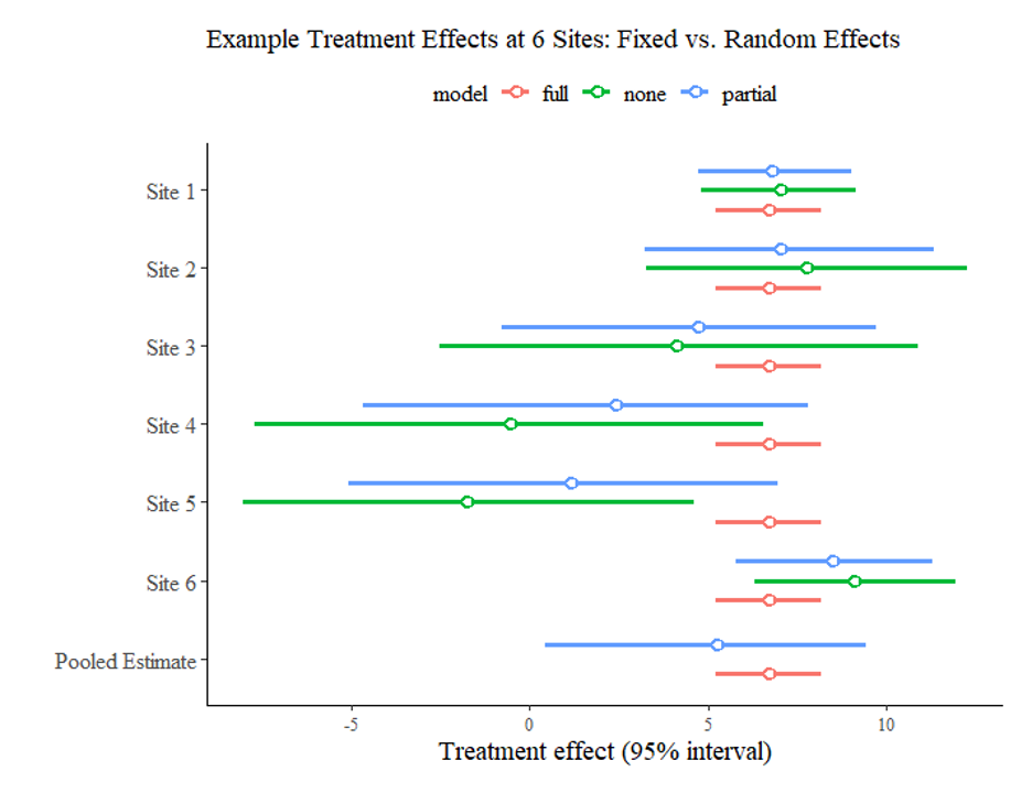
These three columns are all the inputs we need to conduct a simple meta-analysis. The graph below, created using the baggr package in R (Figures 2 and 3), shows estimated treatment effects from each study as estimated separately (“none” in green), as part of a fixed effects model (“full” in red) and as part of a random effects model (“partial” in blue). It also shows overall pooled treatment effects for both full and partial pooling.

Figure 2

library(baggr)
# You can fit Bayesian meta-analysis models in one line of code:
bg_partial <- baggr(data) #partial pooling (baggr default)
bg_full    <- baggr(data, pooling = "full")
bg_none    <- baggr(data, pooling = "none")
# We can easily compare models and plot these comparisons
plot(baggr_compare("partial" = bg_partial,
                   "none" = bg_none,
                   "full" = bg_full)) + 
  ggtitle("Example Treatment Effects at 6 Sites: Fixed vs. Random Effects")

Figure 3

Notably, the estimated treatment effect for each individual study under no pooling is quite different, and in the case of sites 4 and 5, even negative. If we simply estimated a fixed effects model, we would conclude that the intervention has a highly positive effect of more than 5 across the board. However, as the random effects model takes the true heterogeneity in treatment effects across studies into account, its pooled effect estimate is lower, with a wider 95% confidence interval, which includes the true value of 3.

Estimating the model

Random effects models can be estimated using either a frequentist or Bayesian approach. A frequentist approach, likely more familiar to most readers, generally involves some version of maximum likelihood estimation (MLE), which estimates the treatment effect that would make the observed data most likely to have occurred given the specified statistical model. Common statistical software packages for meta-analysis (meta summarize in Stata and metagen in R) use restricted maximum likelihood estimation as the default strategy for random effects models.

Bayesian statistical inference acknowledges that researchers rarely “start from scratch,” knowing nothing about the parameter of interest. We have prior beliefs about values this parameter will likely take, which we can combine with the evidence from newly conducted studies to form posterior beliefs. Estimation using Bayesian inference is implemented in  Stata and R. We use the baggr() command from the baggr package in R.

So which methods should one use—frequentist or Bayesian? This comes down to a trade-off between bias and precision, which stems from the inclusion of prior beliefs in the Bayesian framework. Incorporating prior beliefs potentially increases bias, by introducing information into estimation that is not from the data at hand. Simultaneously, more information, including prior beliefs on treatment heterogeneity, increases precision. This may be especially important when despite a small number of studies, researchers would like to characterize treatment effect heterogeneity rather than only the mean treatment effect. Unlike a systematic review, which may include hundreds of papers, coordinated trials generally have less than ten studies, making Bayesian methods generally more suitable.

Selecting priors

For the Bayesian analysis, we need to set priors for at least two parameters of interest: The underlying mean of the distribution from which study-specific treatment effects are drawn, and the standard deviation of this distribution, that is, how much true treatment effects differ between studies.

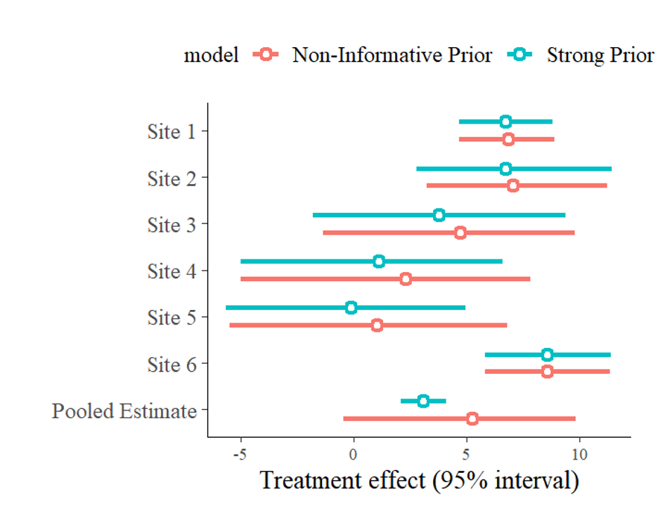
Perhaps the biggest consideration for selecting priors is deciding how informative they should be. The more informative priors are, the more they will affect the results of the estimation. For instance, a prior belief distribution where the treatment effect has an equal chance of taking on any value is not informative (and is called an improper prior) because it adds no information guiding the estimation. Contrarily, a researcher with a strong conviction that the true underlying average treatment effect is approximately 3 could set as their priors, for instance, a normal distribution, with a mean of 3 and a very small standard deviation. This is an example of a strong prior and would bias the parameter estimate toward 3. Figures 4 and 5 show the baggr comparison between these two priors.

Figure 4

non_informative_prior <- baggr(data, prior_hypermean = uniform(-100,100))
strong_prior <- baggr(data, prior_hypermean = normal(3, 0.5))
baggr_compare("Non-Informative Prior"= non_informative_prior, 
              "Strong Prior" = strong_prior, plot=TRUE)

Figure 5

Usually, prior beliefs lie somewhere between these two extremes. In adoption studies, we have a sense of how much adoption may reasonably increase; a relatively light-touch intervention is unlikely to cause a variety used by 1% of farmers at baseline to be adopted by 100% of farmers at endline. Instead, we may predict the variety will be used by, say, 1% to 30% of farmers at endline. A weakly informative prior distribution, which puts relatively less weight on unrealistic outcome values and more weight on more probable outcome values, is ideal.

Introducing (and solving) design complexities

As meta-analysis methods are primarily used for literature reviews, statistical meta-analysis packages do not always have built-in features that accommodate the complexities and richness of individual/household-level data from coordinated trials.

For instance, in the Behavioral Intelligence trials, as is the case in many RCTs, our treatments are randomized at the cluster rather than individual level—hence our estimation must consider that outcomes for observations in a cluster will be naturally correlated. Second, many RCTs do not have just one treatment group; our trials feature a two-by-two factorial design, in which some participants receive no treatment (control), some receive only seed trial packs (treatment 1), some receive only the end-product trial packs/cooking demos (treatment 2), and some receive both treatments (treatment 1 x treatment 2). Finally, we are interested in understanding heterogeneity in treatment effects based on observable characteristics such as the gender of the household head. Hence, we include a small set of covariates in our estimation.

It is possible to estimate a model with all these features with a custom Bayesian model, using another programming language called Stan. Interfaces that can integrate Stan code directly in both Stata and R exist, but acquiring the necessary additional coding language skills may be a significant barrier to conducting a meta-analysis. One of the outputs from the Behavioral Intelligence trials will be an extension of the baggr package to incorporate such design features, which will be available online as a tool for anyone to use.

Conclusion

CGIAR’s extensive expertise in smallholder farming across many crops and regions creates a critical opportunity to use coordinated trials and generate high-quality systematic evidence on what types of innovations can increase agricultural technology adoption. The current consolidation of the CGIAR’s work into Science Programs provides key opportunities to answer questions at a larger scale in a more systematic way using meta-analysis methods. As the Behavioral Intelligence team concludes data collection for their coordinated trials in early 2025, we plan to use the data to run a Bayesian meta-analysis and share findings. We hope the results can serve as an example of the types of high-quality output that can be produced through coordinated trials, and hope to support other teams in completed similar endeavors.

Berber Kramer is a Senior Research Fellow with IFPRI’s Markets, Trade, and Institutions (MTI) Unit; Carly Trachtman is an MTI Associate Research Fellow; Witold Więcek is an independent researcher and statistician. This post is based on research that is not yet peer-reviewed. Opinions are the authors’.

This work was supported by the CGIAR Initiative on Market Intelligence.